Example: HansenLaw

# -*- coding: utf-8 -*-
from __future__ import division
from __future__ import print_function
from __future__ import unicode_literals

import numpy as np
import abel
import matplotlib.pylab as plt

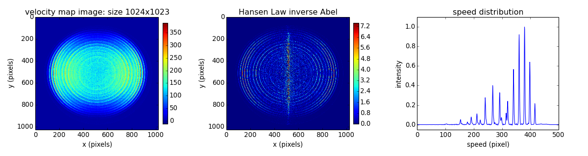
# Hansen and Law inverse Abel transform of velocity-map imaged electrons
# from O2- photodetachement at 454 nm. The spectrum was recorded in 2010
# at the Australian National University (ANU)
# J. Chem. Phys. 133, 174311 (2010) DOI: 10.1063/1.3493349

# load image as a numpy array
# use scipy.misc.imread(filename) to load image formats (.png, .jpg, etc)
print("HL: loading 'data/O2-ANU1024.txt.bz2'")
IM = np.loadtxt("data/O2-ANU1024.txt.bz2")

rows, cols = IM.shape    # image size

# Image center-line should be mid-pixel, i.e. odd number of columns
if cols % 2 == 0:
    print ("HL: even pixel width image, re-adjusting image centre\n"
           "    using `slice` method, returning odd-width size image")
    IM = abel.tools.center.center_image(IM, center="slice", odd_size=True)
    rows, cols = IM.shape   # new image size

# dr=0.5 may help reduce pixel grid coarseness
# NB remember to also pass to angular_integration
AIM = abel.Transform(IM, method='hansenlaw',
                     use_quadrants=(True, True, True, True),
                     symmetry_axis=None,
                     transform_options=dict(dr=0.5),
                     verbose=True).transform

radial, speeds  = abel.tools.vmi.angular_integration(AIM, dr=0.5)

# Set up some axes
fig = plt.figure(figsize=(15, 4))
ax1 = plt.subplot2grid((1, 3), (0, 0))
ax2 = plt.subplot2grid((1, 3), (0, 1))
ax3 = plt.subplot2grid((1, 3), (0, 2))

# raw image
im1 = ax1.imshow(IM, aspect='auto')
fig.colorbar(im1, ax=ax1, fraction=.1, shrink=0.9, pad=0.03)
ax1.set_xlabel('x (pixels)')
ax1.set_ylabel('y (pixels)')
ax1.set_title('velocity map image: size {:d}x{:d}'.format(rows, cols))

# 2D transform
c2 = cols//2   # half-image width
im2 = ax2.imshow(AIM, aspect='auto', vmin=0, vmax=AIM[:c2-50, :c2-50].max())
fig.colorbar(im2, ax=ax2, fraction=.1, shrink=0.9, pad=0.03)
ax2.set_xlabel('x (pixels)')
ax2.set_ylabel('y (pixels)')
ax2.set_title('Hansen Law inverse Abel')

# 1D speed distribution
ax3.plot(radial, speeds/speeds[200:].max())
ax3.axis(xmax=500, ymin=-0.05, ymax=1.1)
ax3.set_xlabel('speed (pixel)')
ax3.set_ylabel('intensity')
ax3.set_title('speed distribution')

# Prettify the plot a little bit:
plt.subplots_adjust(left=0.06, bottom=0.17, right=0.95, top=0.89, wspace=0.35,
                    hspace=0.37)

# save copy of the plot
plt.savefig("example_hansenlaw.png", dpi=100)

plt.show()

(Source code, png, hires.png, pdf)