Three Point

Introduction

The “Three Point” Abel transform method exploits the observation that the value of the Abel inverted data at any radial position r is primarily determined from changes in the projection data in the neighborhood of r. This technique was developed by Dasch [1].

How it works

The projection data (raw data \(\mathbf{P}\)) is expanded as a quadratic function of \(r - r_{j*}\) in the neighborhood of each data point in \(\mathbf{P}\). In other words, \(\mathbf{P}'(r) = dP/dr\) is estimated using a 3-point approximation (to the derivative), similar to central differencing. Doing so enables an analytical integration of the inverse Abel integral around each point \(r_j\). The result of this integration is expressed as a linear operator \(\mathbf{D}\), operating on the projection data \(\mathbf{P}\) to give the underlying radial distribution \(\mathbf{F}\).

When to use it

Dasch recommends this method based on its speed of implementation, robustness in the presence of sharp edges, and low noise. He also notes that this technique works best for cases where the real difference between adjacent projections is much greater than the noise in the projections. This is important, because if the projections are oversampled (raw data \(\mathbf{P}\) taken with data points very close to each other), the spacing between adjacent projections is decreased, and the real difference between them becomes comparable with the noise in the projections. In such situations, the deconvolution is highly inaccurate, and the projection data \(\mathbf{P}\) must be smoothed before this technique is used. (Consider smoothing with scipy.ndimage.filters.gaussian_filter.)

How to use it

To complete the inverse transform of a full image with the hansenlaw method, simply use the abel.transform() function:

abel.transform(myImage, method='three_point', direction='inverse')

Note that the forward Three point transform is not yet implemented in PyAbel.

If you would like to access the Three Point algorithm directly (to transform a right-side half-image), you can use abel.three_point.three_point_transform().

Example

import numpy as np
import matplotlib.pyplot as plt
import abel

n = 101
center = n//2
r_max = 4
r = np.linspace(-1*r_max, r_max, n)
dr = r[1]-r[0]

fig, axes = plt.subplots(ncols = 2)
fig.set_size_inches(8,4)

axes[0].set_xlabel("Lateral position, x")
axes[0].set_ylabel("F(x)")
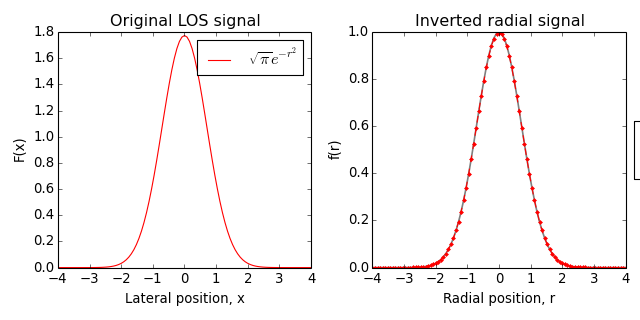
axes[0].set_title("Original LOS signal")
axes[1].set_xlabel("Radial position, r")
axes[1].set_ylabel("f(r)")
axes[1].set_title("Inverted radial signal")

Mat = np.sqrt(np.pi)*np.exp(-1*r*r)
Left_Mat = Mat[:center+1][::-1]
Right_Mat = Mat[center:]
AnalyticAbelMat = np.exp(-1*r*r)
DaschAbelMat_Left = abel.three_point.three_point_transform(Left_Mat)[0]/dr
DaschAbelMat_Right = abel.three_point.three_point_transform(Right_Mat)[0]/dr

axes[0].plot(r, Mat, 'r', label = r'$\sqrt{\pi}e^{-r^2}$')
axes[0].legend()

axes[1].plot(r, AnalyticAbelMat, 'k', lw = 1.5, alpha = 0.5, label = r'$e^{-r^2}$')
axes[1].plot(r[:center+1], DaschAbelMat_Left[::-1], 'r--.', label = '3-pt Abel')
axes[1].plot(r[center:], DaschAbelMat_Right, 'r--.')

box = axes[1].get_position()
axes[1].set_position([box.x0, box.y0, box.width * 0.8, box.height])
axes[1].legend(loc='center left', bbox_to_anchor=(1, 0.5))
fig.tight_layout()
plt.show()

(Source code, png, hires.png, pdf)

Notes

The algorithm contained two typos in Eq (7) in the original citation [1]. A corrected form of these equations is presented in Karl Martin’s 2002 PhD thesis [2]. PyAbel uses the corrected version of the algorithm.

For more information on the PyAbel implementation of the three-point algorithm, please see Issue #61 and Pull Request #64.

Citation

[1] Dasch, Applied Optics, Vol 31, No 8, March 1992, Pg 1146-1152.

[2] Martin, Karl. PhD Thesis, University of Texas at Austin. Acoustic Modification of Sooting Combustion. 2002: https://www.lib.utexas.edu/etd/d/2002/martinkm07836/martinkm07836.pdf