Example: O2 PES PAD

#!/usr/bin/env python
# -*- coding: utf-8 -*-
from __future__ import division
from __future__ import print_function
from __future__ import unicode_literals

import numpy as np
import abel

import matplotlib.pylab as plt
from scipy.ndimage.interpolation import shift

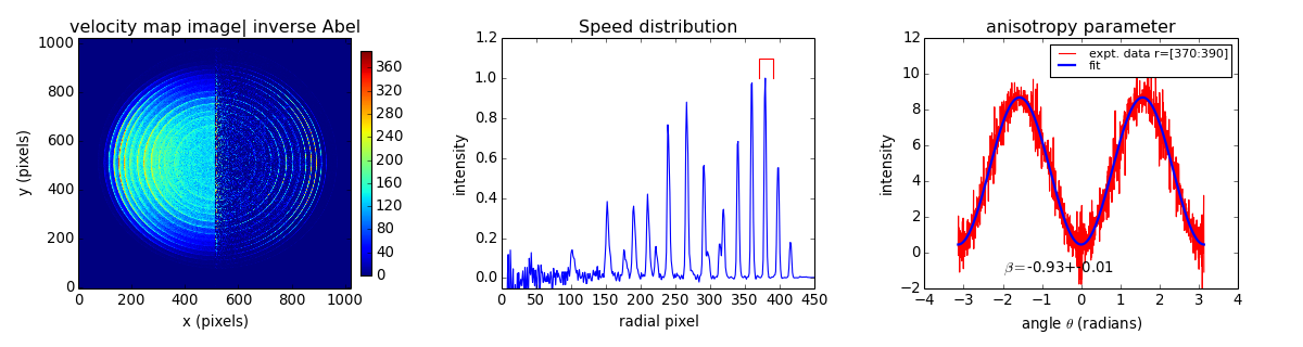
# This example demonstrates Hansen and Law inverse Abel transform
# of an image obtained using a velocity map imaging (VMI) photoelecton
# spectrometer to record the photoelectron angular distribution resulting
# from photodetachement of O2- at 454 nm.
# Measured at  The Australian National University
# J. Chem. Phys. 133, 174311 (2010) DOI: 10.1063/1.3493349

# image file
filename = 'data/O2-ANU1024.txt.bz2'
# numpy handles .gz or plain .txt extensions

# Load image as a numpy array
print('Loading ' + filename)
IM = np.loadtxt(filename)
# use scipy.misc.imread(filename) to load image formats (.png, .jpg, etc)

rows, cols = IM.shape    # image size

# Image center should be mid-pixel, i.e. odd number of colums
if cols % 2 != 1:
    print ("HL: even pixel width image, re-adjusting image centre")
    IM = shift(IM, (-1/2, -1/2))[:-1, :-1]
    rows, cols = IM.shape   # new image size

r2 = rows//2   # half-height image size
c2 = cols//2   # half-width image size
print ('image size {:d}x{:d}'.format(rows, cols))

# Hansen & Law inverse Abel transform
print('Performing Hansen and Law inverse Abel transform:')

AIM = abel.transform(IM, method="hansenlaw", direction="inverse",
                     symmetry_axis=None)['transform']

# PES - photoelectron speed distribution  -------------
print('Calculating speed distribution:')

r, speed  = abel.tools.vmi.angular_integration(AIM)

# normalize to max intensity peak
speed /= speed[200:].max()  # exclude transform noise near centerline of image

# PAD - photoelectron angular distribution  ------------
print('Calculating angular distribution:')
# radial ranges (of spectral features) to follow intensity vs angle
# view the speed distribution to determine radial ranges
r_range = [(93, 111), (145, 162), (255, 280), (330, 350), (350, 370),
           (370, 390), (390, 410), (410, 430)]

# map to intensity vs theta for each radial range
intensities, theta = abel.tools.vmi.calculate_angular_distributions(AIM,
                                                     radial_ranges=r_range)

print("radial-range      anisotropy parameter (beta)")
for rr, intensity in zip(r_range, intensities):
    # evaluate anisotropy parameter from least-squares fit to
    # intensity vs angle
    beta, amp = abel.tools.vmi.anisotropy_parameter(theta, intensity)
    result = "    {:3d}-{:3d}        {:+.2f}+-{:.2f}".format(*rr+beta)
    print(result)

# plots of the analysis
fig = plt.figure(figsize=(15, 4))
ax1 = plt.subplot(131)
ax2 = plt.subplot(132)
ax3 = plt.subplot(133)

# join 1/2 raw data : 1/2 inversion image
vmax = IM[:, :c2-100].max()
AIM *= vmax/AIM[:, c2+100:].max()
JIM = np.concatenate((IM[:, :c2], AIM[:, c2:]), axis=1)
rr = r_range[-3]
intensity = intensities[-3]
beta, amp = abel.tools.vmi.anisotropy_parameter(theta, intensity)
# draw a 1/2 circle representing this radial range
# for rw in range(rows):
#   for cl in range(c2,cols):
#       circ = (rw-r2)**2 + (cl-c2)**2
#       if circ >= rr[0]**2 and circ <= rr[1]**2:
#           JIM[rw,cl] = vmax

# Prettify the plot a little bit:
# Plot the raw data
im1 = ax1.imshow(JIM, origin='lower', aspect='auto', vmin=0, vmax=vmax)
fig.colorbar(im1, ax=ax1, fraction=.1, shrink=0.9, pad=0.03)
ax1.set_xlabel('x (pixels)')
ax1.set_ylabel('y (pixels)')
ax1.set_title('velocity map image| inverse Abel             ')

# Plot the 1D speed distribution
ax2.plot(speed)
ax2.plot((rr[0], rr[0], rr[1], rr[1]), (1, 1.1, 1.1, 1), 'r-')  # red highlight
ax2.axis(xmax=450, ymin=-0.05, ymax=1.2)
ax2.set_xlabel('radial pixel')
ax2.set_ylabel('intensity')
ax2.set_title('Speed distribution')

# Plot anisotropy variation
ax3.plot(theta, intensity, 'r',
         label="expt. data r=[{:d}:{:d}]".format(*rr))


def P2(x):   # 2nd order Legendre polynomial
    return (3*x*x-1)/2


def PAD(theta, beta, amp):
    return amp*(1 + beta*P2(np.cos(theta)))


ax3.plot(theta, PAD(theta, beta[0], amp[0]), 'b', lw=2, label="fit")
ax3.annotate("$\\beta = ${:+.2f}+-{:.2f}".format(*beta), (-2, -1.1))
ax3.legend(loc=1, labelspacing=0.1, fontsize='small')

ax3.axis(ymin=-2, ymax=12)
ax3.set_xlabel("angle $\\theta$ (radians)")
ax3.set_ylabel("intensity")
ax3.set_title("anisotropy parameter")


# Plot the angular distribution
plt.subplots_adjust(left=0.06, bottom=0.17, right=0.95, top=0.89,
                    wspace=0.35, hspace=0.37)

# Save a image of the plot
# plt.savefig(filename[:-7]+"png", dpi=150)

# Show the plots
plt.show()

(Source code, png, hires.png, pdf)