Example: HansenLaw

#!/usr/bin/env python
# -*- coding: utf-8 -*-
from __future__ import division
from __future__ import print_function
from __future__ import unicode_literals

import numpy as np
import abel
import scipy.misc
import matplotlib.pylab as plt

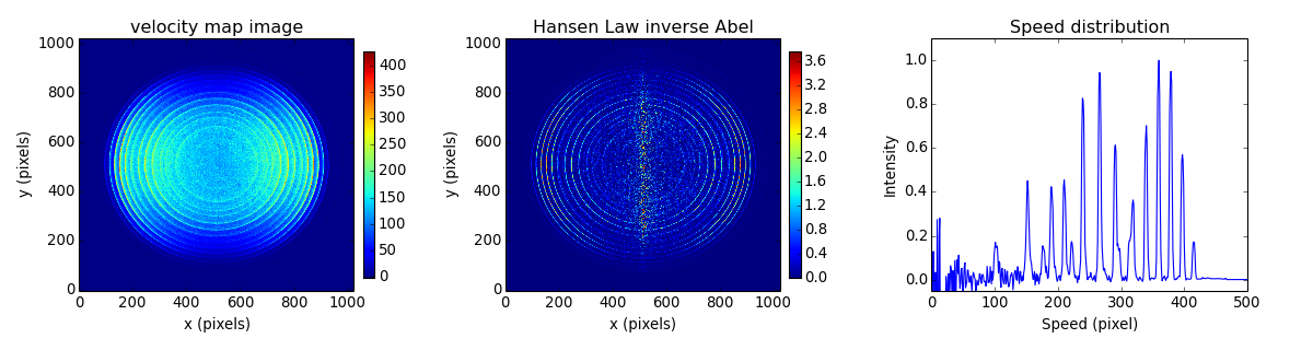
# Hansen and Law inverse Abel transform of a velocity-map image
# O2- photodetachement at 454 nm.
# The spectrum was recorded in 2010
# ANU / The Australian National University
# J. Chem. Phys. 133, 174311 (2010) DOI: 10.1063/1.3493349

# image file in examples/data
filename = 'data/O2-ANU1024.txt.bz2'

# Load as a numpy array
print('Loading ' + filename)
IM = np.loadtxt(filename)
# use plt.imread(filename) to load image formats (.png, .jpg, etc)

rows, cols = IM.shape    # image size

# Image center should be mid-pixel, i.e. odd number of colums
if cols % 2 == 0:
    print ("HL: even pixel width image, re-adjust image centre")
    # re-center image based on horizontal and vertical slice profiles
    # covering the radial range [300:400] pixels from the center
    IM = abel.tools.center.center_image(IM, center="com", odd_size=True)
    rows, cols = IM.shape   # new image size

c2 = cols//2   # half-image
print('image size {:d}x{:d}'.format(rows, cols))

# Step 2: perform the Hansen & Law transform!
print('Performing Hansen and Law inverse Abel transform:')

AIM = abel.transform(IM, method='hansenlaw',
                     use_quadrants=(True, True, True, True),
                     symmetry_axis=None,
                     verbose=True)['transform']

rs, speeds  = abel.tools.vmi.angular_integration(AIM, dr=1)

# Set up some axes
fig = plt.figure(figsize=(15, 4))
ax1 = plt.subplot(131)
ax2 = plt.subplot(132)
ax3 = plt.subplot(133)

# Plot the raw data
im1 = ax1.imshow(IM, origin='lower', aspect='auto')
fig.colorbar(im1, ax=ax1, fraction=.1, shrink=0.9, pad=0.03)
ax1.set_xlabel('x (pixels)')
ax1.set_ylabel('y (pixels)')
ax1.set_title('velocity map image')

# Plot the 2D transform
im2 = ax2.imshow(AIM, origin='lower', aspect='auto', vmin=0,
                 vmax=AIM[:c2-50, :c2-50].max())
fig.colorbar(im2, ax=ax2, fraction=.1, shrink=0.9, pad=0.03)
ax2.set_xlabel('x (pixels)')
ax2.set_ylabel('y (pixels)')
ax2.set_title('Hansen Law inverse Abel')

# Plot the 1D speed distribution
ax3.plot(rs, speeds/speeds[200:].max())
ax3.axis(xmax=500, ymin=-0.05, ymax=1.1)
ax3.set_xlabel('Speed (pixel)')
ax3.set_ylabel('Intensity')
ax3.set_title('Speed distribution')

# Prettify the plot a little bit:
plt.subplots_adjust(left=0.06, bottom=0.17, right=0.95, top=0.89, wspace=0.35,
                    hspace=0.37)

# Save a image of the plot
plt.savefig(filename[:-7]+"png", dpi=150)

# Show the plots
plt.show()

(Source code, png, hires.png, pdf)