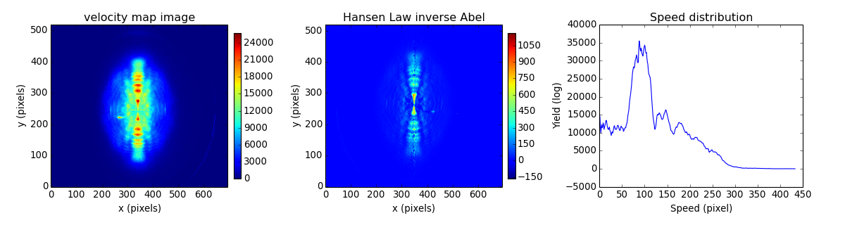
Example: HansenLaw Xenon

#!/usr/bin/env python
# -*- coding: utf-8 -*-

from __future__ import absolute_import
from __future__ import division
from __future__ import print_function
from __future__ import unicode_literals

import numpy as np
import matplotlib.pyplot as plt

import abel
import scipy.misc

# This example demonstrates Hansen and Law inverse Abel transform
# of an image obtained using a velocity map imaging (VMI) photoelecton
# spectrometer to record the photoelectron angular distribution resulting
# from photodetachement of O2- at 454 nm.
# This spectrum was recorded in 2010
# ANU / The Australian National University
# J. Chem. Phys. 133, 174311 (2010) DOI: 10.1063/1.3493349

# Before you start, centre of the NxN numpy array should be the centre
#  of image symmetry
#   +----+----+
#   |    |    |
#   +----o----+
#   |    |    |
#   + ---+----+

# Specify the path to the file
#filename = 'data/O2-ANU1024.txt.bz2'
filename = 'data/Xenon_ATI_VMI_800_nm_649x519.tif'

# Name the output files
name = filename.split('.')[0].split('/')[1]
output_image = name + '_inverse_Abel_transform_HansenLaw.png'
output_text  = name + '_speeds_HansenLaw.dat'
output_plot  = name + '_comparison_HansenLaw.pdf'

# Step 1: Load an image file as a numpy array
print('Loading ' + filename)
#im = np.loadtxt(filename)
im = plt.imread(filename)
(rows,cols) = np.shape(im)
print ('image size {:d}x{:d}'.format(rows,cols))


# Step 2: perform the Hansen & Law transform!
print('Performing Hansen and Law inverse Abel transform:')

recon = abel.transform(im, method="hansenlaw", direction="inverse",
                       symmetry_axis=None, verbose=True, center=(240,340))['transform']

r, speeds = abel.tools.vmi.angular_integration(recon)


# save the transform in 8-bit format:
#scipy.misc.imsave(output_image,recon)

# save the speed distribution
#np.savetxt(output_text,speeds)

## Finally, let's plot the data

# Set up some axes
fig = plt.figure(figsize=(15,4))
ax1 = plt.subplot(131)
ax2 = plt.subplot(132)
ax3 = plt.subplot(133)

# Plot the raw data
im1 = ax1.imshow(im, origin='lower', aspect='auto')
fig.colorbar(im1, ax=ax1, fraction=.1, shrink=0.9, pad=0.03)
ax1.set_xlabel('x (pixels)')
ax1.set_ylabel('y (pixels)')
ax1.set_title('velocity map image')

# Plot the 2D transform
im2 = ax2.imshow(recon, origin='lower', aspect='auto')
fig.colorbar(im2, ax=ax2, fraction=.1, shrink=0.9, pad=0.03)
ax2.set_xlabel('x (pixels)')
ax2.set_ylabel('y (pixels)')
ax2.set_title('Hansen Law inverse Abel')

# Plot the 1D speed distribution
ax3.plot(speeds)
ax3.set_xlabel('Speed (pixel)')
ax3.set_ylabel('Yield (log)')
ax3.set_title('Speed distribution')
#ax3.set_yscale('log')

# Prettify the plot a little bit:
plt.subplots_adjust(left=0.06, bottom=0.17, right=0.95, top=0.89, wspace=0.35,
                    hspace=0.37)

# Save a image of the plot
plt.savefig(output_plot, dpi=150)

# Show the plots
plt.show()

(Source code, png, hires.png, pdf)